How to add filter to column in excel (Step-by-Step)

Excel Filter, also known as AutoFilter, is a convenient approach to show only the data that is important at the time and hide all other data. In Excel spreadsheets, you may filter rows by value, format, and criteria. You may copy, modify, chart, or print only visible rows after applying a filter without rearranging the full list.

How to apply filter in excel online, 2016 and 2019

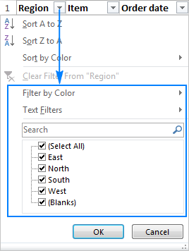
1. To filter a column, click the drop-down arrow next to it.

2. To easily deselect all data, uncheck the Select All box.

3. Click OK after checking the boxes next to the data you wish to see.

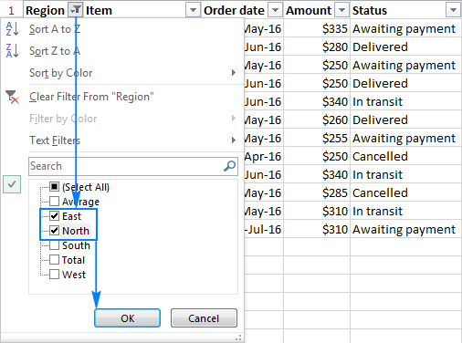
This is how, for example, we may filter data in the Region column to see just sales from the East and North:

4. Done! Any areas other than East and North are temporarily hidden by the filter, which is applied to column A.

The Filter button Filter button replaces the drop-down arrow in the filtered column, and hovering over that button shows a screen tip indicating which filters are applied

How to filter numbers in excel

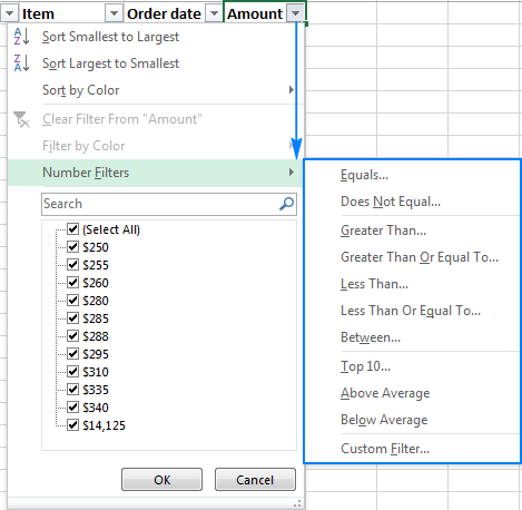
1. Filter numbers that are either equal to or not equal to a specific number.

2. Filter for numbers that are greater than, less than, or equal to the provided values.

3. Top ten or bottom ten numbers are filtered.

4. Cells with numbers that are above or below the average should be filtered.

5. The image below depicts the whole set of number filters available in Excel.

To establish a filter that only shows orders between $250 and $300, for example, follow these steps:

1. In the column header, click the autofilter arrow and navigate to Number Filters.

2. Choose an appropriate comparison operator from the drop-down menu, such as Between... in this case.

3. Fill out the lower bound and higher bound settings in the Custom AutoFilter dialogue box. Excel proposes using the comparison operators Greater than or equal to and Less than or equal to. If you don't want the threshold values to be included, simply modify them to Greater than and Less than.

4. Press Ok.

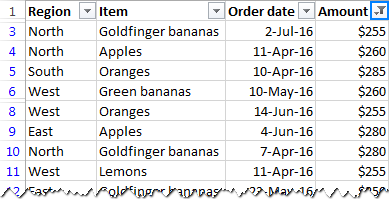
5. As a result, only orders worth $250 to $300 are displayed:

Note: 

To get the newest version of WPS Office, you must first access this operating interface. This was an attempt to teach you about how to add filters in excel on windows. You can access “insert the columns” in all versions of Excel, be it 2016, 2019, online, on windows or on Mac. If you want to access different styles and designs of bar charts and pie charts, you need to have access of WPS Premium, without that you cannot access them.

You just need to have a little understanding of how and which way things work and you are good to go. With having this basic knowledge or information of how to use it, you can also access and use different other options on excel or spreadsheet. Also, it is very similar to Word or Document. So, in a way, if you learn one thing, like Excel, you can automatically learn how to use Word as well because both of them are very similar in so many ways. If you want to know more about WPS Office, you can download WPS Office to access, Word, Excel, PowerPoint for free.