In the world of spreadsheets, Google Sheets function formulas are essential for performing complex calculations, data manipulation, and automation. However, many people struggle to understand these formulas and need a comprehensive guide to overcome the challenges they face. This guide aims to provide a solution by introducing Google Sheets functions and common formulas, offering an overview, examples, syntax explanations, and practical usage scenarios. By delving into this guide, readers can gain the knowledge and confidence to effectively utilize Google Sheets' function formulas and unlock its full potential for their data-related tasks.
Part 1. 13 Essential Google Sheets Formulas and How to Use them

In this section, we will explore 13 essential Google Sheets formulas that are vital for data manipulation and analysis. From the basic SUM formula for adding values to the versatile VLOOKUP formula for searching and retrieving data, each formula will be explained with clear instructions and practical examples. By mastering these essential formulas, you'll be equipped to optimize your workflow and make the most of Google Sheets' powerful features.. Here are a few examples:
1. SUM:
Adds the values within a range of cells.

Choose the cell in which the sum should appear.
Select the range of cells you want to add, then type “=SUM(“.
Close the parentheses and press Enter.
2. VLOOKUP:
Calculates the sum of two values and outputs the result.
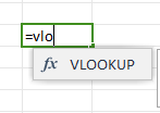
Choose the cell in which the lookup result should be displayed.
Type "=VLOOKUP(" and provide the lookup value, the range to search in, the column index for the result, and whether to find an exact match or approximate match.
Close the parentheses and press Enter.
3. AVERAGE:
Calculates the average of a range of cells.

Choose the cell in which the average should appear.
Type "=AVERAGE(" and then select the range of cells you want to average.
Close the parentheses and press Enter.
4. COUNT:
Counts the number of cells with numerical values.

Choose the cell in which the count should display.
Select the range of cells you wish to count after typing “=COUNT(“.
Close the parentheses and press Enter.
5. MIN:
Determines the minimum value in a range.

Choose the cell in which the minimum value should be displayed.
Type "=MIN(" and then select the range of cells you want to find the minimum from.
Close the parentheses and press Enter.
6. MAX:
Finds the maximum value in a range.
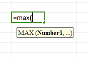
Pick the cell that should show the highest value.
Type "=MAX(" and then select the range of cells you want to find the maximum from.
Close the parentheses and press Enter.
7. IF:
Performs conditional evaluations and returns different results based on the condition.

Select the cell where you want the result of the IF statement to appear.
Type "=IF(" and provide the condition to check, the value if true, and the value if false.
Close the parentheses and press Enter.
8. CONCATENATE:
Combines text strings from multiple cells into one.
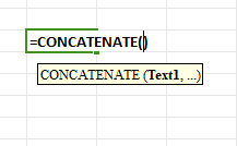
Select the cell where you want the concatenated text to appear.
Type "=CONCATENATE(" and then provide the text or cell references you want to join together.
Close the parentheses and press Enter.
9. DATE:
Creates a date value based on the provided year, month, and day.
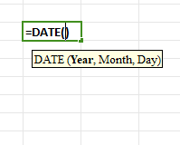
Select the cell where you want the date to appear.
Type "=DATE(" and provide the year, month, and day as separate arguments or cell references.
Close the parentheses and press Enter.
10. TODAY: Retrieves the current date.

Choose the cell that will contain the current date.
Type "=TODAY()".
Press Enter.
11. MID:
The MID function allows you to extract a specified number of characters from a text string, starting from a specified position. It is useful when you want to extract a specific segment of text within a larger string.
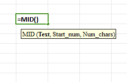
Select the cell where you want the extracted text to appear.
Type "=MID(" and provide the cell reference or text, the starting position, and the number of characters to extract.
Close the parentheses and press Enter.
12. LEFT:
The LEFT function extracts a specified number of characters from the beginning (left) of a text string.

Select the cell where you want the left portion of text to appear.
Type "=LEFT(" and provide the cell reference or text and the number of characters to extract from the left.
Close the parentheses and press Enter.
13. RIGHT:
The RIGHT function extracts a specified number of characters from the end (right) of a text string.
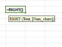
Select the cell where you want the right portion of text to appear.
Type "=RIGHT(" and provide the cell reference or text and the number of characters to extract from the right.
Close the parentheses and press Enter.
By mastering these formulas, you can streamline your data analysis, automate calculations, and gain valuable insights. Practice and experimentation will further enhance your proficiency with Google Sheets formulas.
Part 2. Alternative to google sheets -WPS Spreadsheet

WPS Spreadsheet serves as an excellent alternative to Google Sheets, offering a range of features and functionalities that enhance your productivity and data management. Here's a brief introduction to WPS Spreadsheet and its key functions:
Free and Comprehensive Editing: WPS is a free software that allows you to edit Word, Excel, and PowerPoint files without any subscription fees. With WPS, you can seamlessly work on documents, spreadsheets, and presentations, providing a complete office suite solution.
Convenient PDF Function: WPS goes beyond traditional spreadsheet software by offering a dedicated PDF function. Once you download and install WPS, you gain access to membership benefits, including the ability to convert various PDF documents effortlessly.
Formula Mastery with Free Tutorials: WPS Spreadsheet understands the importance of formulas in data analysis. That's why it provides free tutorials that guide you in mastering formulas, enabling you to perform complex calculations and unlock deeper insights from your data.
Experience the power of WPS Spreadsheet as it combines the convenience of free editing, versatile PDF capabilities, and valuable formula tutorials. Embrace an alternative solution that empowers your data-driven endeavors.
With WPS Spreadsheet, you have access to a powerful and versatile toolset that enables seamless editing of different file formats, including PDFs. Additionally, the availability of free tutorials ensures that you can expand your knowledge and proficiency in using formulas within WPS Spreadsheet.
Discover the capabilities of WPS Spreadsheet and experience a user-friendly and feature-rich alternative to Google Sheets.
FAQs About google sheets formulas
Q1: What are the main formulas of Google Sheets?
The main formulas of Google Sheets include SUM, AVERAGE, COUNT, MAX, MIN, VLOOKUP, IF, CONCATENATE, DATE, and TODAY. These formulas help perform calculations, search for data, combine text, and work with dates.
Q2: How do you use Google sheet functions?
To use Google Sheets functions, start with an equal sign (=) followed by the function name and its arguments. Provide the necessary inputs, such as cell references or values, within parentheses. Press Enter to get the result.
Q3: What is unique formula in Google Sheets?
The UNIQUE formula extracts unique values from a range or array in Google Sheets. Simply type "=UNIQUE(" followed by the range or array, close the parentheses, and press Enter. The cell will display the distinct values, removing any duplicates.
Google Sheets formulas are essential for data manipulation, analysis, and automation.
Conclusion
In conclusion, this article provided an overview of 13 essential Google Sheets formulas, equipping users with the knowledge to manipulate and analyze data effectively. Additionally, the article emphasized the benefits of using WPS Office as an alternative to Google Sheets, highlighting its free editing capabilities for Word, Excel, and PowerPoint files, as well as its PDF function and helpful tutorials. By incorporating these formulas and considering WPS Office, users can enhance their data management and productivity in various contexts.


