Removing the last character from a string in Excel can be beneficial for data cleaning, formatting, and analysis. However, it can be challenging to accurately identify the last character, especially with varying data formats. This article will share 5 easy ways to remove the last character in Excel.
How to Remove Last Character from String Excel
1. Use of REPLACE Function
Step 1: Set Up Formula
Select an empty cell, like C5.
Step 2: Enter Formula
In C5, type: =REPLACE(B5,9,1," ")
B5 is the source.
Start after the desired part (e.g., "Jane Doe").
Replace one character ("*") with a space (" ").
Step 3: Execute Formula
Press ENTER. Cell C5 will display the modified text.

Step 4: Repeat
For other cells, follow steps 1-2, adjusting start_num and num_chars:

Original: John Smith#
Modified: John Smith
2. Combine LEFT and LEN Functions
Step 1: Choose a Cell
Pick an empty cell, such as C5.
Step 2: Apply the Formula
In C5, type: =LEFT(B5, LEN(B5) - 1)
The LEN function finds total characters minus one.
The LEFT function captures characters from the start.
Step 3: Execute the Formula
Press ENTER. C5 will display the modified text.

Step 4: Extend the Method
Drag the Fill Handle to apply the formula to other cells.

3. Use of VBA
Step 1: Open VBA Editor
Press ALT+F11 to access Microsoft Visual Basic.

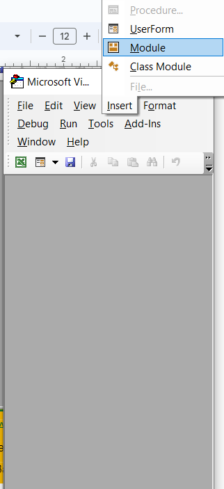
Step 2: Create a Module
In the Visual Basic window, go to Insert > Module.
Step 3: Insert VBA Macro Code
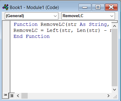
Paste the following code in the module:
Function RemoveLC(str As String, num_chars As Long)
RemoveLC = Left(str, Len(str) - num_chars)
End Function
Step 4: Apply the Formula
In the worksheet, enter =@RemoveLC(B5,1).
B5 is the text string.
1 represents the number of characters to remove.

Step 5: Execute the Formula
Press ENTER to remove the last character from the text.

Step 6: Extend the Method
Drag the Fill Handle to apply the formula to other cells.

4. Use of Flash Fill Option
Step 1: Select Adjacent Cell
Click on an adjacent cell (C5) next to the entry in the dataset.
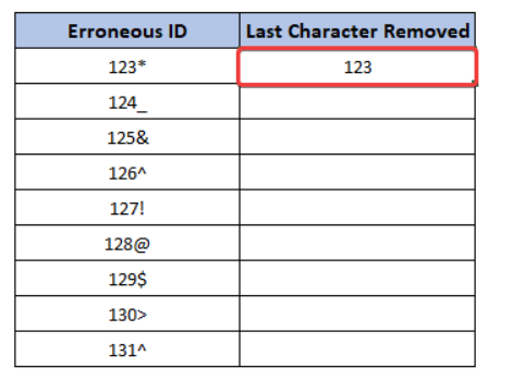
Step 2: Type Modified Entry
Type the first entry without the unnecessary character.
Step 3: Apply Flash Fill
Press ENTER, then go to Data Tab > Flash Fill (in Data Tools section).

Step 4: Select Flash Fill
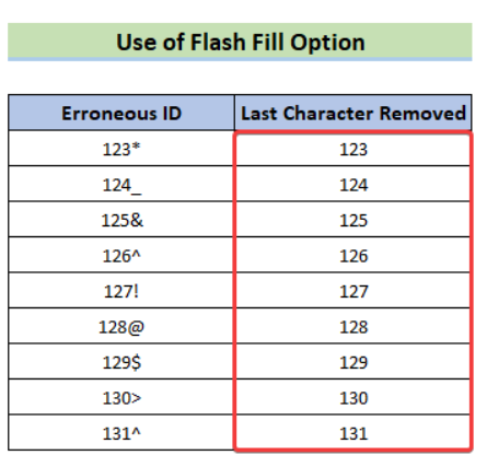
Click on the Flash Fill option. All the number values will appear, excluding the last character..
5. Combine VALUE, LEFT and LEN Functions
Step 1: Insert the Formula
Insert the formula below into any blank cell (C5):
=VALUE(LEFT(B5,LEN(B5)-1))
Step 2: Press ENTER
Press ENTER to execute the formula. The last unnecessary character will be removed from the cell B5.
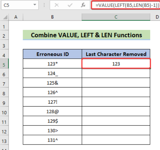
Step 3: Apply to Other Cells
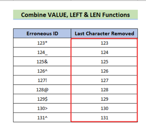
Drag the Fill Handle down to apply the formula to other cells. This will remove the last character from each entry, resulting in a data shape like the image below.
Free Office Suite for Word, Excel, PowerPoint ——WPS Office

WPS Office is a comprehensive software suite comprising four essential components: Writer, Spreadsheet, Presentation, and PDF. It proudly touts its compatibility with popular formats including Microsoft Office, Google Docs, and Adobe PDF. Moreover, WPS Office extends its reach across diverse platforms, encompassing Windows, macOS, Linux, Android, and iOS.
Pros
Data Cleaning: Effortlessly enhance data quality by eliminating unwanted first characters, ensuring accuracy.
String Manipulation: Easily manipulate strings to fit your needs, refining data presentation and analysis.
Data Transformation: Transform data for various purposes, tailoring it to your specific requirements.
Improved Data Handling: Navigate Excel tasks with enhanced efficiency, streamlining processes for better results.
If you are looking for a free office suite that can help you with your data cleaning needs, I would recommend WPS Office. It is a great option for students, businesses, and anyone else who needs to work with data. Download WPS Office for free today and elevate your Excel capabilities to new heights!
Download Website: https://www.wps.com/
Frequently Asked Questions (FAQs)
1. What is the Excel function for the last position of character in string?
To locate the last occurrence of a specific character within a string and extract the content to its right, utilize the RIGHT function combined with FIND and SUBSTITUTE. Formulate the equation as follows:
=RIGHT(A2,LEN(A2)-FIND("@",SUBSTITUTE(A2,"/","@",LEN(A2)-LEN(SUBSTITUTE(A2,"/",""))),1))
2. How do I use the MID Function for variable length strings?
For extracting portions of variable-length strings, such as a website name amidst double forward slashes (//) and .com, employ the MID function. Craft the formula like so:
=MID(A2,FIND("//",A2)+2,FIND(".com",A2,10)-FIND("//",A2)-2)
3. How to compare multiple cells in Excel?
When comparing cells, ignoring case, a straightforward formula like the one below works: =A1=B1
The result will be either TRUE or FALSE, indicating whether the cells match or not. For more customized outputs, such as displaying "Equal" or "Not equal," utilize the IF function: =IF(A1=B1, "Equal", "Not equal")
Conclusion
In conclusion, these five methods are essential Excel formatting tips that make removing the last character from strings effortless. By using functions like REPLACE, LEFT, LEN, VBA, and Flash Fill, you can effectively clean up your data and enhance its usability.
Furthermore, the introduction of WPS Office provides an additional tool for data management. With its range of features for data transformation, string manipulation, and data cleaning, it offers a valuable resource for anyone working with Excel.
